Spatial Queries
In this exercise, we are trying to solve a number of problems in which spatial data plays a role. The exercise attempts to bring you the intuition required to solve spatial problems within a database context. If you pay attention, you will see that much of this mimicks solving spatial problems through a GIS. The interface and the language is different but much of the spatial intuition is the same. The purpose of this exercise is threefold:
- ❶ – Create a conceptual model with geometric primitives,
- ❷ – Understand the extension mechanisms of UML, and
- ❸ – Apply the Model Driven Architecture design approach.
This exercise is organised in two parts. The first part (this section) aims at refreshing your SQL knowledge and allows you to familiarise with spatial queries. The second part (next section) challenges you to define a number of queries for a given set of problems.
The Data
The data that we will be using in these exercises is organised in separate schemas inside the gimla_exercises database as follows:
netherlands.municipality → statistical data at municipal level.
Attribute descriptions municipality relation (relevant attributes only)
| gm_code | municipal code |
| gm_naam | name of the municipality as defined by city council |
| aantal_hh | number of private households |
| aant_inw | number of inhabitants [absolute, figures are rounded off] |
| aant_man | number of men [absolute, figures are rounded off] |
| aant_veouw | number of women [absolute, figures are rounded off] |
| opp_tot | total municipal area (including water bodies) in hectares (ha) |
| opp_land | land area in hectares (ha) |
| opp_water | surface water area in hectares (ha) |
| bev dichth | population density per square kilometer |
| p_hh_m_k | percentage of households with children |
| p_hh_z_k | percentage of households without children |
| gem_hh_gr | average household size [absolute] as the number of persons living in private households divided by the number of private households. |
| oad | average number of properties per square kilometer |
| geom | political boundary represented as a MultiPolygon using the Dutch National Reference System (Amersfoort/RD New) |
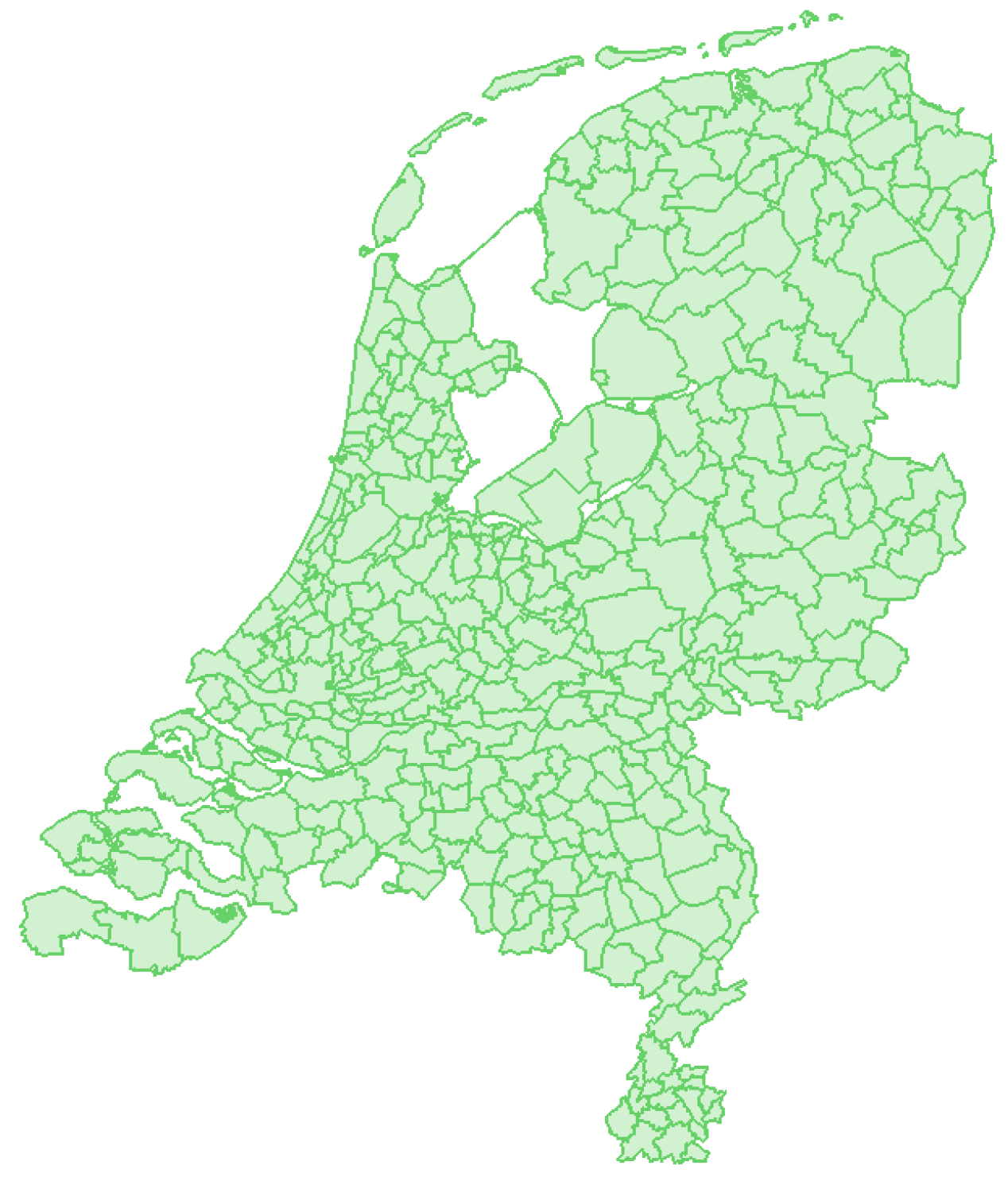
netherlands.neighbourhood → statistical data at neighbourhood level.
Attribute descriptions neighbourhood relation (relevant attributes only)
| bu_code | code of the neighbourhood |
| bu_naam | name of the neighbourhood |
| geom | political boundary represented as a MultiPolygon using Amersfoort/RD New coordinates |
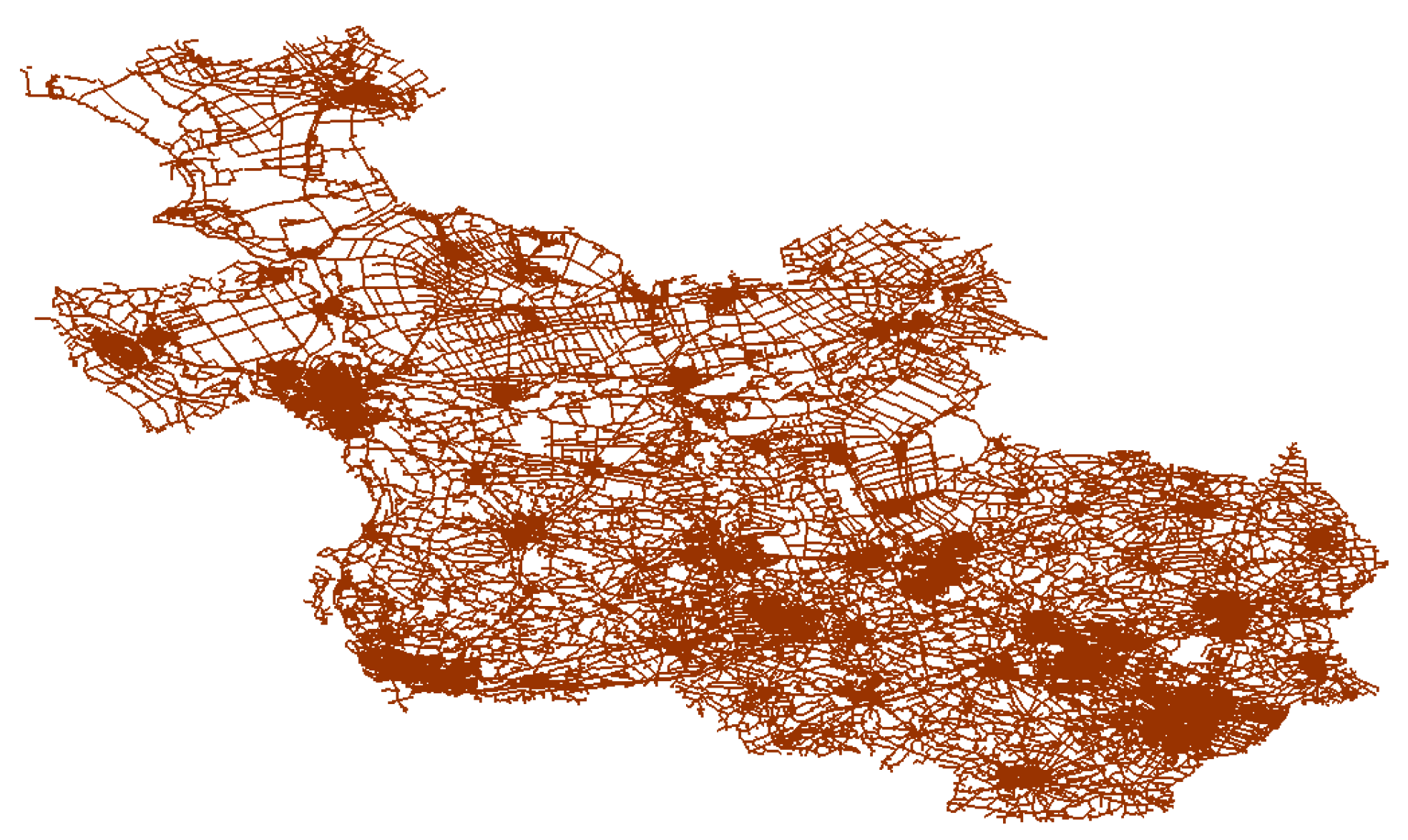
netherlands.road_ov → road segments for the province of Overijssel extracted from OpenStreetMap.
Attribute descriptions netherlands.road_ov
| roadname | road name |
| refcode | highway name |
| roadtype | road type |
| oneway | direction type (1=oneway) |
| bridge | bridge lane (1=bridge) |
| maxspeed | speed limit |
| province | province code |
| provname | province name |
| provabbr | province abbreviation |
| nation | country code |
| cntryname | country name |
| cntryabbr | country abbreviation |
| geom | geometry of the road segments represented as a MultiLineString using WGS84 |
netherlands.builtup_area → settled areas, or urban areas, around the country
Attribute descriptions builtup_area relation (relevant attributes only)
| bu_area_code | code of the urbanized area |
| bu_area_name | name of the urbanized area |
| prov_code | code of the province where the urbanized area is located |
| geom | urban area extent represented as a Polygon using Amersfoort/RD New coordinates |
europe.country → political division of countries in Europe.
Attribute descriptions country relation (relevant attributes only)
| gid | unique identifier of the country |
| nation | country code |
| cntryname | official English name of the country |
| cntryabb | abbreviation of the country name |
| geom | geometry of the political boundary represented as a MultiPolygon in WGS84 |
europe.admin_area→ Statistical data on population of the 1st level administrative divisions of countries in Europe.
Attribute descriptions admin_area relation (relevant attributes only)
| gid | unique identifier of the country |
| provname | official English name of the province |
| cntryname | official English name of the country |
| population | number of inhabitants |
| geom | geometry of the administrative boundary represented as a MultiPolygon in WGS84 |
europe.builtup_area → Major European settlements.
Attribute descriptions builtup_area relation (relevant attributes only)
| gid | unique identifier of the built-up area |
| area_name | official English name of the built-up area |
| geom | geometry of the surface covered by the built-up area represented as a MultiPolygon in WGS84 |
Familiarization
To get familiar with the available data, we will do some simple queries. This will help you get acquinted with these new tables but more importantly with the spatial capabilities of the database. Remember to use the online PostgreSQL/PostGIS manual for insights on any of the function definitions and correct query formulations.
In conformance with the Simple Features for SQL (SFSQL) specification, PostGIS provides two tables to track and report on the geometry types available in a given database. The first table, spatial_ref_sys, defines all the spatial reference systems known to the database and will be described in greater detail later. The second table, geometry_columns, provides a listing of all “features” (defined as an object with geometric attributes), and the basic details of those features. 1 shows how we can use that view to list all existing geometric attributes in the database.
|
1 2 3 4 |
GeomColumns ≡ SELECT * FROM geometry_columns; |
- The result will include all existing geometry columns (attributes) in the database with their corresponding table name, schema name, data type, SRID and dimension.
The following query determines the type of geometry values that are stored or allowed in a geometry field of a particular table. We use the table builtup_area for the example. The function we require here is ST_GeometryType. We simply use the geometry column name as the parameter for the function (see 2).
|
1 2 3 4 5 |
GeomType ≡ SELECT ST_GeometryType(b.geom) FROM netherlands.builtup_area AS b LIMIT 1; |
We saw in the lectures that a MultiPolygon object is formed by a number of LinearRings, each representing a separate polygon. The next example determines the number of rings (polygons) in a given geometry. The function required here is ST_NRings as shown in 3.
|
1 2 3 4 5 |
MunicipalPolygons ≡ SELECT ST_NRings(m.geom) FROM netherlands.municipality AS m WHERE m.gm_naam = 'Dronten'; |
Queries like this and certainly all spatial queries can be formulated using math. Note that the schema name can not be made part of the math formulation as schema names are only an structural artifact in the database.
$\hspace{0.6cm}\mathrm{MunicipalPolygons}\equiv\{\,m\in municipality\mid{}m.gm\_naam=\mathrm{'Dronten'}\bullet{}st\_nrings(m.geom)\,〛$
The previous two examples used so-called Geometry Accessor functions. The following example uses a so-called Geometry Output functions (check the PostGIS manual for details in both types of functions).
|
1 2 3 4 5 |
GeomAsText ≡ SELECT ST_AsText(b.geom) FROM netherlands.builtup_area AS b LIMIT 5; |
- In this case the ST_AsText function retrieves the geometry property of an object in text format. An arbitarry limit has been used just to retrieve only 5 records.
The next (and last) example is a little bit more elaborated as it operates on two tables, enschede.busstop and netherlands.neighbourhood, and makes use of a spatial join to relate the two tables. The idea of this query is to find out which neighbourhood contains the bus station called Graeshoek.
|
1 2 3 4 5 6 7 |
StationNeighbourhood ≡ SELECT b.station_name, n.bu_naam AS neighborhood_name, n.bu_code AS neighborhood_code FROM netherlands.neighbourhood AS n JOIN enschede.busstop AS b ON ST_Contains(n.geom, ST_Transform(b.geom,28992)) WHERE b.station_name = 'Graeshoek'; |
- Note that since the geometry attributes of the two sets of objects are in different reference systems, one of them needs to be transformed before the join can be realised.
Revisit Early Queries
During the math exercises we queried the tables employee and department using their address or general location. If you look carfully at those two tables, you will notice that both, employees and department objects, have a geometric property. Most probably the addreses have been geocoded. This combined with the newly acquired knowledge gives us the oportunity to execute some spatial analysis on these objects. For example we can generate the coordinates of the address where Maria P. Tersteeg lives.
|
1 2 3 4 5 6 |
CoordsMariaTersteeg ≡ SELECT e.fname || ' ' || e.lname AS full_name, ST_X(e.home) AS x_coord, ST_Y(e.home) AS y_coord FROM employee AS e WHERE e.ssn = 987654321; |
The new knowledge available to you shows you how spatial functions bring an additional level of functionality to the database and allow us to execute either simple to sophicticated spatial analysis. It is now time for you to try a few queries yourself.
Determine which employees live within 6 kilometeres of the headquaters.
Find out which employee lives closest to his/her own supervisor.
Detemine which employee lives the nearest to the University of Twente.
What is the distance in kilometeres between offices?