Web Maps 2: Python Services

Thus far we have been using OpenLayers JavaScript to add mapping functionality to the page, and in separate exercises you learned how to use Geo-Webservices (using MapServer) and consume these in a OpenLayers map client. You also learned how to create Python services, and used one to include a dynamic version of a bar chart. Now we will continue to also add a Python service to create a Thematic Map of the same data of country the provinces we used in the bar chart. We could go search for an OWS service that produces what we need, but instead we are going to create our own Python service. The mechanism necessary for this task is a so-called 'server-side script', written in CGI Python. If you have never used Python to create a CGI script before, make sure to first do the exercise we have created to introduce you to that...!

You might have also done the exercise on how to use scripts with a so-called REST interface. Using REST services falls outside the scope of this exercise, but you are of course welcome to add a REST interface to your services here also...!

Vector Layers using Python services

The data we need for the map service is the same we used for the bar chart, the world.prov_pop table of the exercises database. We need to generate data that can be used as input for the OpenLayers javascript library to map this on top of the OpenStreetMap layer. The most obvious data format to use for this is GeoJSON.

GeoJSON is a format in which simple geometry is expressed in JSON syntax. GeoJSON supports the geometry types Point, LineString, Polygon, MultiPoint, MultiLineString, and MultiPolygon. Geometric objects with additional attributes/properties are Feature objects. Sets of features are contained by FeatureCollection objects. It is an IEEE standard: http://geojson.org/. In Python any JSON, so also GeoJSON, is essentially a Dictionary. GeoJSON is supported by almost all GIS software, including OpenLayers.

The listing below shows an SQL query that can be used to generate the data of the provinces for the service as a GeoJSON output.

We do not explain all the parts of the SQL here, but note that we use the PostGres built-in functions json_build_object() and json_agg() to aggregate the rows selected into a valid GeoSJON Feature Collection. The geometry of the provinces is converted from the internal PostGIS binary to GeoJSON, using the ST_AsGeoJSON function in line 7. The jsonbset function in line 6 is there to avoid the geometry ending up as a long text description in the properties of each Feature: That would be superfluous as the geometry will already be encoded as a GeoJSON geometry.

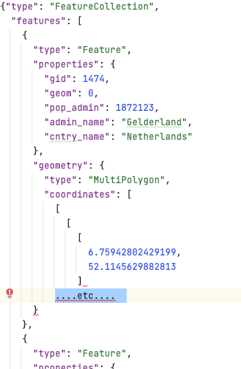
Run the query using pgAdmin to see it in action. The result should be similar in content to figure 1 below (it will be unformatted, to get that and the syntax-highligthing you'd have to load it into an 'intelligent' editor such as Notepad++ or PyCharm).

We are now ready to work on the service script. Proceed to create a new file using the code in Listing 2, and save it as /student/<<SNUMBER>>/services/provinces.py.

The provinces.py script first loads necessary modules: cgi to be able to act as a CGI application, json for handling JSON objects, psycopg2 for connecting to Postgres DB's. Next, it connects to the DB and runs the query. Finally the results containing the geometries are sent back to the client in JSON format [33–35]. It is important to state the appropriate content-type for the response, as we do in line 33, so that the content of the response can be parsed properly by the client application.

Test the new script in your browser to verify that it works.

Those of you that payed attention, would probably think: "could this not also be achieved by using a WFS...?" And they'd be correct! By using the MapServer's WFS capability to create GeoJSON output we'd have achieved the same result. We chose to use a Python service, because this is easier to parameterize later, as you will find out in the Challenge section...

Now that we have a service in place, we can use it to overlay the boundaries of Dutch provinces on the map. Our new service does not use a standard OGC service request/response structure (such as in a WFS), but it does however generate a data stream which is fully compliant, a correct GeoJSON object. We can therefore use OpenLayers to consume the service. Update the simple-website/scripts/viewer.js by adding the highlighted code below at the end:

To render the provinces layer, we have defined a new layer using OpenLayers ol.layer.Vector object (in line 3-12). One of the vector object's properties is url, which we use to load the data from the service we just created. The response data is structured as GeoJSON, so we use this as the format definition for the vector data [6]. As part of the format object we define the projection in which the original data is, EPSG:4326, and then the projection to be used for display, EPSG:3857 [7-8]. OpenLayers will take care of executing the corresponding transformation. Finally we specify a display name for this layer [11], and then add it to the map [13].

Reload the page to see how the polygons of the provinces are drawn on the map. Now the provinces are shown in a default style as we have not specified any style ourselves. To fix that, we just need to create, and use, a style object. Insert the following code in the simple-website/scripts/viewer.js file

Now we should have a more attractive provinces layer. If you refresh the page the result should look like the image in the figure below.

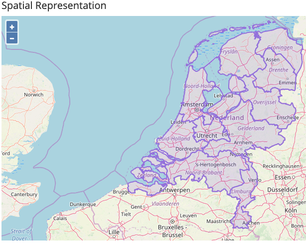
However, the map may not be as nicely zoomed in to the Netherlands as we show here. The user can do that of course using the OpenLayers zoom tools, but it would be nice if the system does that... This can be achieved by using the mapView.fit() function of OpenLayers (see line 8 in the listing below). But because the loading and rendering of the data is an asynchronous process, we need to wait a bit until the loading is completed. That is achieved by running the fitting function as the result of a so-called callback promise: the promise .once is fulfilled once the 'change' event has happened (line 6):

Now we have a web site that consumes various services. But they do so only for The Netherlands (or whatever other country you have hard-coded in your Python services SQL queries)... The next and last section contains an optional challenge: to create a parameterized version where the users can make their own choice of country to show the map and bar chart for.