Data Services
Based on the requirements of the use case we have to decide what type of statistical data will be displayed in the application. Two decisions are required, one the administrative unit level, and two, the type of statistical data. After a careful analysis on the available data, the choice has been made to use Districts administrative level and population and landuse as variables.
This means we will need to have access to the descriptive data of the districts (name, code, etc.); to the geometry of the districts, both as basemap and as features; to the population values of each district; and, to the landuse per district including type and area covered. Figure 3-1 depicts a conceptual representation of the data form the point of view of the application.

The source data for the application has been stored in a PostgreSQL/PostGIS server, which can be access with the following parameters:
Server: gisedu.itc.utwente.nl Port: 5432 Database: exercises Schema: netherlands
Go ahead an check the schema to familiarise with the data. Figure 3-2 depicts a PSM model including only the tables and attributes relevant for our application. Check carefully the attributes and relationships so that it is clear that the structure in which the data is stored differs from the structure in which the data is needed by thh application.

The PSM model depicted in Figure 3-2 shows that the landuse table has two landuse type attributes for the year 2012, class_2012 and group_2012. Both of them associated with the class_code attribute of the landuse_class table. A quick check to the tables and their attributes reveals that group_2012 stores values for aggregated landuse types, which have single digit identifiers, and that class_2012 stores values for disaggregated landuse types. Presumably the suffix 2012 indicates the year for which the values are valid. The PSM model also shows that both tables districts and landuse have geometric attributes. It is important to understand the spatial relationships between those two types of polygon geometries to be able to decide how to generated the data needed by the application. Figure 3-3 depicts both districts polygons (orange) and landuse polygons (grey). Analyse the spatial relationship to determine how to generate landuse areas and percentages, per land use type, per district, as depicted in the model in Figure 3-1.

To satisfy the needs of the application, our next task is, to create one OGC service for serving the district polygons, and one REST service to deliver district population and landuse data.
WMS & WFS Service
The OGC service is more or less straightforward as we do not need any sort of data manipulation to produce the required output. The only real task here is to create the configuration file with the necessary content to deliver the data via MapServer. For this purpose we need a configuration file. Proceed to create the CityApp/app/api/adminboundaries.map file using the code in Listing 3-1.
|
1 2 3 4 5 6 7 8 9 10 11 12 13 14 15 16 17 18 19 20 21 22 23 24 25 26 27 28 29 30 31 32 33 34 35 36 37 38 39 40 41 42 43 44 45 46 47 48 49 50 51 52 53 54 55 56 57 58 |
MAP NAME "Dutch Adminisrative Boundaries" IMAGECOLOR 255 255 255 TRANSPARENT ON SIZE 1700 1700 #--- PROJECTION "init=epsg:28992" END #--- EXTENT -90000 290000 430000 630000 #----- Start of WEB DEFINITION ------ WEB IMAGEPATH "/ms4w/tmp/ms_tmp/" IMAGEURL "/ms_tmp/" #--- METADATA "map" "d:/iishome/student/SSNUMBERR/CityApp/app/api/adminboundaries.map" "ows_schemas_location" "http://schemas.opengeospatial.net" "ows_title""Dutch adminisrative boundaries at various levels." "ows_abstract" "WMS & WFS with Dutch administrative boundaries. Data from CBS www.cbs.nl" "ows_onlineresource" "https://gisedu.itc.utwente.nl/cgi-bin/mapserv.exe?" "ows_fees""None" "ows_accessconstraints" "None" #--- "wms_contactperson" "SDI-T Team" "wms_contactorganization" "ITC" "wms_addresstype" "Postal" "wms_address" "Hengelosestraat 99" "wms_city" "Enschede" "wms_stateorprovince" "Overijssel" "wms_postcode" "7514 AE" "wms_country" "The Netherlands" "wms_title" "WMS service of Dutch Adminisrative Boundaries" "wms_srs" "EPSG:4326 EPSG:28992 EPSG:3857 EPSG:3044" "wms_feature_info_mime_type" "application/vnd.ogc.gml" "wms_feature_info_mime_type" "text/plain" "wms_feature_info_mime_type" "text/html" "wms_server_version" "1.1.1" "wms_formatlist""image/png,image/gif,image/bmp,image/jpeg" "wms_format" "image/png" "wms_enable_request" "GetMap GetFeatureInfo GetCapabilities" #--- "wfs_title" "WFS service of Dutch Adminisrative Boundaries" "wfs_srs" "EPSG:4326 EPSG:28992 EPSG:3857 EPSG:3044" "wfs_server_version" "1.0.0" "wfs_namespace_prefix" "cbs" "wfs_enable_request" "GetFeature DescribeFeature GetCapabilities" END END #----- End of WEB DEFINITION ------ #----- Start of LAYER DEFINITIONS ------ #----- End of LAYER DEFINITIONS ------ END |
Not much to explain here, the code in Listing 3-1 defines all the metadata elements required when implementing compliant OGC services. One thing though, just make sure to use your actual SNUMBER in line 19.
To generate the content for the service, we have to write the corresponding SQL code to get the data from the database, and then include that code as part of the layer definition for districts in the configuration file. Since this is a straightforward query we will do both, define the query and configure the district layer in on go. Update the CityApp/app/api/adminboundaries.map file, using the code in Listing 3-2.
|
1 2 3 4 5 6 7 8 9 10 11 12 13 14 15 16 17 18 19 20 21 22 23 24 25 26 27 28 29 30 31 32 33 34 35 36 37 38 39 40 41 42 43 44 45 46 47 48 49 50 51 52 53 54 55 56 57 58 59 60 61 62 63 64 65 66 67 68 69 70 |
dotdotdot "wfs_srs" "EPSG:4326 EPSG:28992 EPSG:3857 EPSG:3044" "wfs_server_version" "1.0.0" "wfs_namespace_prefix" "cbs" "wfs_enable_request" "GetFeature DescribeFeature GetCapabilities" END END #----- End of WEB DEFINITION ------ #--- OUTPUTFORMAT NAME "geojson" DRIVER "OGR/GEOJSON" MIMETYPE "application/json; subtype=geojson" FORMATOPTION "STORAGE=stream" FORMATOPTION "FORM=SIMPLE" END #--- #----- Start of LAYER DEFINITIONS ------ #----- districts layer ----- LAYER NAME "districts" TYPE POLYGON STATUS ON DUMP TRUE #--- CONNECTIONTYPE postgis CONNECTION "user=exercises password=exercises host=gisedu.itc.utwente.nl port=5432 dbname=exercises options='-c client_encoding=UTF8'" DATA "ogc_geom FROM (SELECT gid AS ogc_id, wk_code AS district_code, regexp_replace(wk_name, 'Wijk (.. )', '') AS district_name, geom AS ogc_geom FROM netherlands.district WHERE gm_naam LIKE '%CITYNAME%') AS query USING UNIQUE ogc_id USING SRID=28992" #--- VALIDATION "default_CITYNAME" "%" "CITYNAME" ".+$" END #--- PROJECTION "init=epsg:28992" END #--- METADATA "wms_title" "Dutch Districts" "wms_abstract" "Administrative level between Municipality and Neighbourhood." "wms_include_items" "all" "wfs_title" "Dutch Districts" "wfs_abstract" "Administrative level between Municipality and Neighbourhood." "wfs_getfeature_formatlist" "geojson" "gml_featureid" "ogc_id" "gml_include_items" "all" END #--- CLASS NAME "district" STYLE OUTLINECOLOR 130 60 255 WIDTH 1 END END OPACITY 60 END #----- districts layer ----- #----- End of LAYER DEFINITIONS ------ END |
We have now specified a layer object in the configuration file to respond to WMS or WFs request for districts 23–68. We have also defined an additional output format that the WFS response is not only available as GML but also as GeoJSON 12–19. The SQL code used to extract the data from the database includes a runtime variable called CITYNAME, which can be used to retrieve only the districts of a given municipality if needed 33–37. It is now time to test the service. paste the request code shown below in the address bar of your browser to send a GetCapabilities request and then check the results. As always, replace the placeholder in the example request with your own SNUMBER.
https://gisedu.itc.utwente.nl/cgi-bin/mapserv.exe?SERVICE=WFS&VERSION=1.1.0&MAP=d:/iishome/student/<<SNUMBER>>/CityApp/app/api/adminboundaries.map&REQUEST=GetCapabilities
If all went well, you should also be able to send a GetFeature request. An example request is shown bellow. Figure 3-4 shows an example of the response to the request.
https://gisedu.itc.utwente.nl/cgi-bin/mapserv.exe?SERVICE=WFS&VERSION=1.1.0&MAP=d:/iishome/student/<<SNUMBER>>/CityApp/app/api/adminboundaries.map&REQUEST=GetFeature&TYPENAME=districts&SRS=EPSG:28992&MAXFEATURES=2
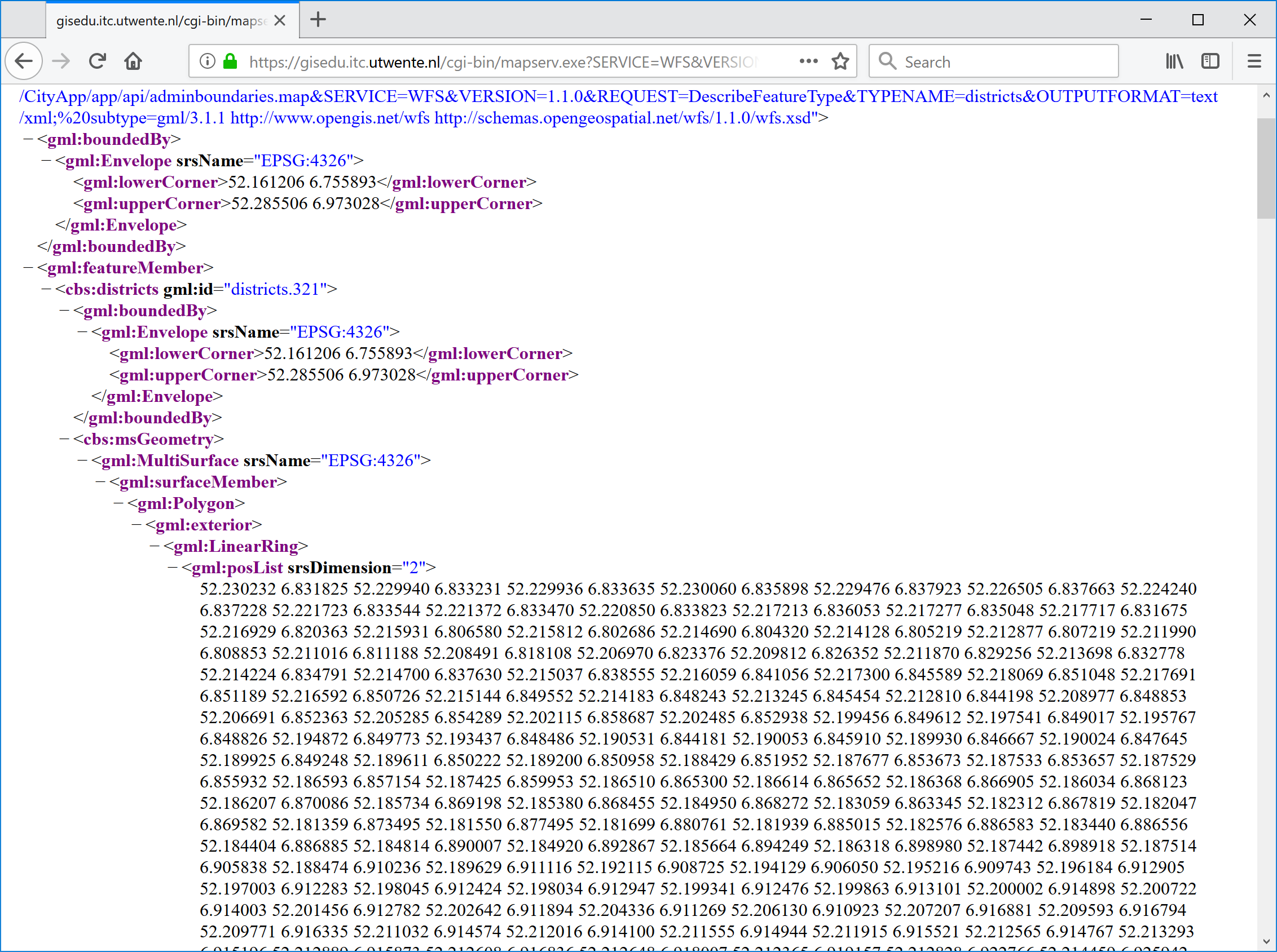
If your browser does not show similar results to those in Figure 3-4, then go back to check what could have gone wrong. Use the listings as a reference for your analysis. If things went well, we can say that the OGC service required for the application is ready. Time to move on to the REST service now.
REST Service
For this service, we have to engineer the SQL code to generate the output required by the application. If you studied Figures 3-1 and 3-3 carefully, you would know that we need to determine the intersection between landuse polygons and district polygons. You would also know that the web application is not interested in the resulting geometry of that intersection but in its area, so we need to make sure to produce that as an output. We cannot assume that every type of landuse appears only once inside each district. This means, we also need to ensure that multiple instances of the same landuse type inside a district are grouped together for the area calculation. We know that there are two attributes for landuse types, in this case we will use the aggregated attribute, group_2012, which has only nine different classes. Certainly for each tuple in the output we also want some district details, such as, its name, code, etc. Let's pit all of these conditions together in a SQL statement. Start pgAdmin an run the code in Listing 3-3. Check the code carefully to determine which part of it corresponds to which of the conditions stated above. For now, we will assume that we are doing this for the municipality of Enschede. This way we have an example value to use in the filter expression of the queries.
|
1 2 3 4 5 6 |
-- Compute the area of landuse (in m2) per landuse type in each disctrict in Enschede SELECT d.wk_code, d.wk_name, l.group_2012, sum(St_Area(ST_Intersection(l.geom, d.geom))) AS use_m2 FROM netherlands.landuse AS l JOIN netherlands.district AS d ON ST_Intersects(l.geom, d.geom) WHERE d.gm_naam = 'Enschede' GROUP BY 1,2,3 ORDER BY 1,2; |
The server needed about nine seconds to produce the output, which is not bad, but also not good enough for a Web Service. Users will fall asleep if they have to wait that long for a service response. And this output does not yet look like the model in Figure 3-1. We need a way out. There are various possibilities, but this is nor the place neither the time to discuss them (query optimization falls weel outside the scope of this exercise), so what we will do is to store the results in an intermediate table, and then use that as table a source for the service. Use the code in Listing 3-4 to create the new table. There is no need to have both, the district code and the district name in this table, so we will only store the district code. Use the SQL code in lines 14–15 to check the result of the table creation process.
|
1 2 3 4 5 6 7 8 9 10 11 12 13 14 15 |
-- Q1 -- -- Create a table for the results of the landuse type areas in each district in Enschede -- This way we get a faster response to web service requests CREATE TABLE SSNUMBERR.landuse_per_district AS MMSSGG002 SELECT d.wk_code, d.wk_name, l.group_2012, sum(St_Area(ST_Intersection(l.geom, d.geom))) AS use_m2 FROM netherlands.landuse AS l JOIN netherlands.district AS d ON ST_Intersects(l.geom, d.geom) WHERE d.gm_naam = 'Enschede' GROUP BY 1,2 ORDER BY 1,2; -- Q2 -- -- Check that indeed the correct data content has been generated SELECT wk_code, group_2012, use_m2 FROM SSNUMBERR.landuse_per_district; MMSSGG002 |
This operation could have been done for the whole country, but it will take time, so for now, we only run it for the area we need which is 'Enschede'. If you need to do this for another municipality just reuse this code, but remember that the table will already exist, so you need to use INSERT INTO rather than CREATE, to add the new records.
With the nine plus seconds removed from the equation, we can continue with the process of generating the output that fits the structure of the Web service (see Figure 3-1). We already have the area in square meters covered by each landuse type in every district, but we also need to know the percentage of that landuse with respect to the area of the district itself. For that computation we need to join the new table, again, with the districts table as shown in Listing 3-5.
|
1 2 3 4 5 6 7 8 9 |
-- Combining district data with landuse data SELECT l.wk_code, 'g' || group_2012 AS group, round(use_m2::NUMERIC,2) AS m2, round((use_m2 * 100 / ST_Area(d.geom))::NUMERIC,2) AS pct FROM SSNUMBERR.landuse_per_district AS l JOIN netherlands.district AS dMMSSGG002 ON (l.wk_code = d.wk_code) WHERE d.gm_naam = 'Enschede' ORDER By 1,2; |
This output now contains landuse data as specified in the model in Figure 3-1. Having said that, if we look at the result carefully, say the first six or seven records you will notice that this query does not generate records for landuse groups that do not exist in a specific district, which is quite logical. to make correct visualisations however, we need one record for each of the nine landuse groups in every district. Since those missing records simply do not exist, we need to force them into the output. To that end, we can create a cartesian product between the nine landuse groups and the districts, and then use that result in the JOIN, with the landuse per district data. Let's check if this will work. Listing 3-6 shows, first, the code for the cartesian product 4–6. And then, how that is used in the join with the landuse data 12–19. Go ahead and run both queries to see what is going on. In testing the new approach, we have only used the minimum possible number of attributes in the output.
|
1 2 3 4 5 6 7 8 9 10 11 12 13 14 15 16 17 18 19 |
-- Q1 -- -- Generation of rows for all combinations of landuse groups and districts, -- namely a cartesian product SELECT d.wk_code, 'g' || generate_series(1,9) AS group FROM netherlands.district AS d WHERE d.gm_naam = 'Enschede'; -- Q2 -- -- Checking that the district-landuse_group pairs approach using a cartesian product, -- actually works (see Figure 12) WITH cp AS ( SELECT d.wk_code, 'g' || generate_series(1,9) AS group FROM netherlands.district AS d WHERE d.gm_naam = 'Enschede' ) SELECT cp.wk_code, cp.group, l.use_m2 FROM cp LEFT JOIN SSNUMBERR.landuse_per_district AS l MMSSGG002 ON (cp.wk_code = l.wk_code) AND ('g' || l.group_2012 = cp.group); |
Figure 3-5 shows that the cartesian product, in combination with a LEFT JOIN command used in the query 18, has done the trick. A normal join would not have sufficed here. The output now contains nine records for every district, and, if any of the districts does not have any landuse of a type, the value in the use_m2 attribute for that combination contains a NULL value. Great!.

Since the approach worked nicely, let's then use it for real. Listing 3-7 shows the updated SQL code, including the attributes required to produce the percentage attribute.
|
1 2 3 4 5 6 7 8 9 10 11 12 13 14 |
-- Producing the required landuse data for all districts WITH cp AS ( SELECT d.wk_code AS code, 'g' || generate_series(1,9) AS group, st_area(d.geom) / 1000000 AS area_km2 FROM netherlands.district as d WHERE d.gm_naam = 'Enschede' ORDER BY 1,2 ) SELECT cp.code, cp.group, round(l.use_m2::NUMERIC,2) AS m2, round((l.use_m2 * 100 / (cp.area_km2 * 1000000))::NUMERIC,2) AS pct FROM cp LEFT JOIN jmmg.landuse_per_district as l ON (l.wk_code = cp.code) AND ('g' || l.group_2012 = cp.group); |
Now we are able to generate the landuse data in a form that will allow proper visualization is the browser. It sounds good, but we are not there yet. If we revisit the model in Figure 3-1, we see that the landuse data (landuse_2012) is to be delivered as an array, and not as individual records for every district. The reason for that is that the district record itself needs other attributes, including, population, name, etc. Like always there are many paths to follow here, however since we are going to deliver the data in JSON format, we can choose to convert the landuse records into a JSON array
|
1 2 3 4 5 6 7 8 9 10 11 12 13 14 15 16 17 |
-- Grouping all the landuse data by districts WITH cp AS ( SELECT d.wk_code AS code, 'g' || generate_series(1,9) AS group, st_area(d.geom) / 1000000 AS area_km2 FROM netherlands.district as d WHERE d.gm_naam = 'Enschede' ORDER BY 1,2 ) SELECT cp.code, json_agg(( cp.group, round(l.use_m2::NUMERIC,2), round((l.use_m2 * 100 / (cp.area_km2 * 1000000))::NUMERIC,2) )) AS landuse_2012 FROM cp LEFT JOIN SSNUMBERR.landuse_per_district as l MMSSGG002 ON (l.wk_code = cp.code) AND ('g' || l.group_2012 = cp.group) GROUP BY 1; |
Figure 3-6 shows the result of our latest query step. This time the output has one attribute with the district code and one attribute with an array of landuse data values, exactly as we need. Unfortunately, the SQL command that we have available to create the array, does not allow us to control the name of the variables inside the JSON object. What we get in the output as variable names is: "f1", "f2", etc. This is unfortunate but not necessarily a big problem. There is nothing we can do about it right now, but we certainly have to keep this in mind and repair it later on.

It seems, the only thing left to do in terms of the content of the output, is to add the other requiered attributes for every district. Listing 3-9 shows the code of the query that generates the output required by the application, form the source data as available in the database.
|
1 2 3 4 5 6 7 8 9 10 11 12 13 14 15 16 17 18 19 20 |
-- Putting it all together, districts statistical data WITH cp AS ( SELECT d.wk_code AS code, 'g' || generate_series(1,9) AS group, substring(d.wk_code from 7 for 2) AS label, regexp_replace(d.wk_name, 'Wijk (.. )', '') AS name, d.aant_inw::REAL AS pop_2016, st_area(d.geom) / 1000000 AS area_km2 FROM netherlands.district as d WHERE d.gm_naam = 'Enschede' ORDER BY 1,2 ) SELECT cp.code, cp.label, cp.name, cp.pop_2016, cp.area_km2, json_agg(( cp.group, round(l.use_m2::NUMERIC,2), round((l.use_m2 * 100 / (cp.area_km2 * 1000000))::NUMERIC,2) )) AS landuse_2012 FROM cp LEFT JOIN SSNUMBERR.landuse_per_district as l MMSSGG002 ON (l.wk_code = cp.code) AND ('g' || l.group_2012 = cp.group) GROUP BY 1,2,3,4,5; |
This result is very nice, but as we know, no Web application can directly execute database commands, we need to create a server-side script and make it responsible for: listening to client requests, executing the corresponding query, and sending the response back to the client. As such, the next step in our service creation process, is to create the script and include in it the SQL code that we have just engineered. Besides the query, the script needs to be able to connect to the database and also has to encode the result of the query in JSON. Insert the code in Listing 3-10 into the file CityApp/app/api/districtstats.py, which will serve as the Web service script. Do not forget to create the necessary folder structure to place the file at the right location.
|
1 2 3 4 5 6 7 8 9 10 11 12 13 14 15 16 17 18 19 20 21 22 23 24 25 26 27 28 29 30 31 32 33 34 35 36 37 38 39 |
# Generate district statistics (population and landuse) import os import json import psycopg2 from psycopg2.extras import RealDictCursor print ("Content-type: application/json") print () file = open(os.path.dirname(os.path.abspath(__file__)) + "\pg.credentials") connection_string = file.readline() + file.readline() pg = psycopg2.connect(connection_string) records_query = pg.cursor(cursor_factory=RealDictCursor) records_query.execute(""" WITH cp AS ( SELECT d.wk_code AS code, 'g' || generate_series(1,9) AS group, substring(d.wk_code from 7 for 2) AS label, regexp_replace(d.wk_name, 'Wijk (.. )', '') AS name, d.aant_inw::REAL AS pop_2016, st_area(d.geom) / 1000000 AS area_km2 FROM netherlands.district as d WHERE d.gm_naam = 'Enschede' ORDER BY 1,2 ) SELECT cp.code, cp.label, cp.name, cp.pop_2016, cp.area_km2, json_agg(( cp.group, round(l.use_m2::NUMERIC,2), round((l.use_m2 * 100 / (cp.area_km2 * 1000000))::NUMERIC,2) )) AS landuse_2012 FROM cp LEFT JOIN SSNUMBERR.landuse_per_district as l MMSSGG002 ON (l.wk_code = cp.code) AND ('g' || l.group_2012 = cp.group) GROUP BY 1,2,3,4,5; """) results = json.dumps(records_query.fetchall()) results = results.replace('"f1"','"group"').replace('"f2"','"m2"').replace('"f3"','"pct"') print ('{"success":"true", "districts":',results,'}') |
The structure of this script is as follows: In lines 2–5, all required modules are included. The output format of the service is prepared in lines 7–8. Then, in lines 10–12 the database connection is prepared using an external credential file, which we will create next. In lines 14–35 we assigned the query prepared earlier to a variable. Next, the query is executed and parsed as JSON 37. In line 38 we repair the variable names in the JSON object, by replacing the names created by the Postgres array function, with the correct names according to our service schema. Finally, in line 39 the results are dispatch back to the client application requesting the data.
Include the content of file Listing 3-11 in the file CityApp/app/api/pg.credentials. This file is used by the Web service script to connect to the database. As in all the scripts for we use the user exercises which has read-only access to the content of the database, even to your own tables.
|
1 |
dbname='exercises' host='gisedu.itc.utwente.nl' port='5432' user='exercises' password='exercises' |
We should now be ready to test the service. Head to your Web browser and use the request URL below to check the behaviour of the service. If there is no response, check the console to find out what could be the problem and proceed to repair it.
https://gisedu.itc.utwente.nl/student/<<SNUMBER>>/CityApp/app/api/districtstats.py
The response of the service was as expected, so we could declare this task completed. There is however one additional step to take care off. If you revise the service script, you will notice that we have hardcoded the city name 23. If we were to leave it like this, then we might as well call the service 'enschededistricts. To avoid this behaviour, we need to adapt the script so that the client application that uses the service can pass on the municipality name as a parameter. To that end, update the file CityApp/app/api/districtstats.py as shown in Listing 3-12.
|
1 2 3 4 5 6 7 8 9 10 11 12 13 14 15 16 17 18 19 20 21 22 23 24 25 26 27 28 29 30 31 32 33 34 35 36 37 38 39 40 41 42 43 44 45 |
# Generate district statistics (population and landuse) import os import psycopg2 import json import cgi from psycopg2.extras import RealDictCursor print ("Content-type: application/json") print () params = cgi.FieldStorage() cityName = params.getvalue('cityname') if cityName is None: cityName = '' file = open(os.path.dirname(os.path.abspath(__file__)) + "\pg.credentials") connection_string = file.readline() + file.readline() pg = psycopg2.connect(connection_string) records_query = pg.cursor(cursor_factory=RealDictCursor) records_query.execute(""" WITH cp AS ( SELECT d.wk_code AS code, 'g' || generate_series(1,9) AS group, substring(d.wk_code from 7 for 2) AS label, regexp_replace(d.wk_name, 'Wijk (.. )', '') AS name, d.aant_inw::REAL AS pop_2016, st_area(d.geom) / 1000000 AS area_km2 FROM netherlands.district as d WHERE d.gm_naam = '%s' ORDER BY 1,2 ) SELECT cp.code, cp.label, cp.name, cp.pop_2016, cp.area_km2, json_agg(( cp.group, round(l.use_m2::NUMERIC,2), round((l.use_m2 * 100 / (cp.area_km2 * 1000000))::NUMERIC,2) )) AS landuse_2012 FROM cp LEFT JOIN SSNUMBERR.landuse_per_district as l MMSSGG002 ON (l.wk_code = cp.code) AND ('g' || l.group_2012 = cp.group) GROUP BY 1,2,3,4,5; """ % (cityName)) results = json.dumps(records_query.fetchall()) results = results.replace('"f1"','"group"').replace('"f2"','"m2"').replace('"f3"','"pct"') print ('{"success":"true", "districts":',results,'}') |
Study an understand the changes that were made to the script. Test the modified service with a new request including the new parameter. Below you find an example request.
https://gisedu.itc.utwente.nl/student/<<SNUMBER>>/CityApp/app/api/districtstats.py?cityname=Enschede
The script is now capable of handling request for different municipalities. Figure 3-7 shows the response of the request using 'Enschede' as a value for the 'cityname' parameter. Try other city names to make sure that the script actually works (study the output carefully).
